Tree based models in R on Titanic Data
This is the first time I blog my journey of learning data science, which starts from the first kaggle competition I attempted - the Titanic. In this competition, we are asked to predict the survival of passengers onboard, with some information given, such as age, gender, ticket fare…

Translated letter reveals first hand account of the “unforgettable scenes where horror mixed with sublime heroism” as the Titanic sank Photo: Getty Images
How bad is this tragedy?
Let’s take some exploratory data analysis to look at the big picture of the tragedy. Looking at the bar charts, we can find that there is a rough estimation of 38% survival rate for the Titanic passengers. Much bigger percentage of male passengers were perished than females. The proportion of the First, Second and Third class are about 25%, 25% and 50%. The third class passengers are much more vulnerable. The Titanic has a variety of decks range from top deck (T) to bottom deck (G). The passengers on different decks seems indifferent in comparing the survival likelihood. 
Some other facts
The majority of passengers on-board are adults, whose age range from 20-40. There a spike in survived portion for children and another spike in perished portion of young people from 20-30 years old. Ticket fares are mainly distributed below 50£ and the passengers with cheaper ticket fare are prone to die. 
Decision Tree
Derived from decision tree method, Decision Tree learning/model recursively divides the predictors so that the misclassification error of the outcome will eventually be reduced to a certain level, which is defined as complexity parameter (cp). There are two types of decision tree models: 1) classification tree: used for classification problem, which has a discrete outcome 2) regression tree: used for regression problem, which has a continuous outcome The big advantage of the decision tree model is the interpretability. By looking at the decision tree diagram, the passengers without title ‘Dr’,’Mr’,’Rev’,’Sir’ and Pclass =1,2 are the most likely to survive (21% of the passengers fall under this category), while the passengers without title ‘Dr’,’Mr’,’Rev’,’Sir’, Pclass=3 and FamilySize<4.5 are the most likely to perish (with 0.9% misclassification error). Decision Tree model is prone to overfit the problem, if we are greedy to choose a complex model, in order to reach a high accuracy. Comparing the relative simple model (cp=0.01) with complex model (cp=0.005), simple model has fewer splitting nodes, easier to understand but has a error of 1%. However the complex model has more nodes, but the error is reduced to 0.5%.

Decision Tree (cp=0.01)
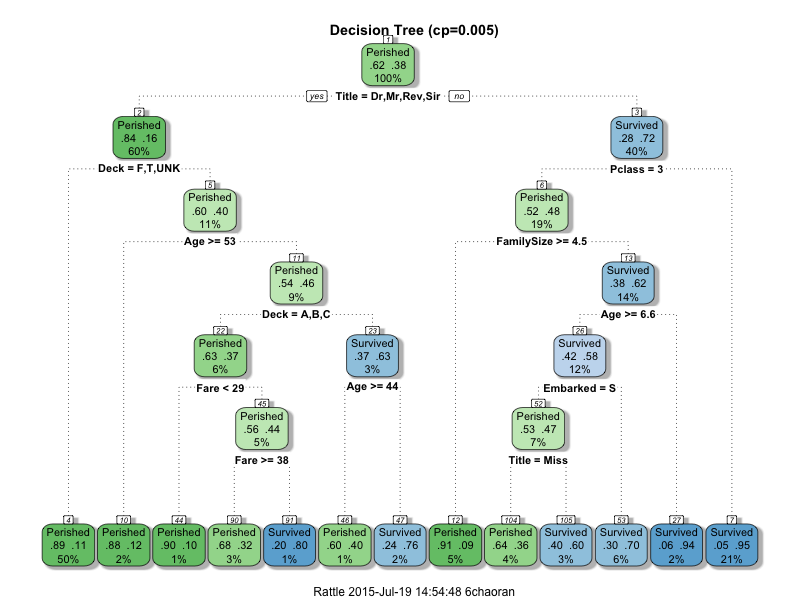
Decision Tree (cp=0.005)
Tree Pruning
Over-fitting (high variance) and Under-fitting (high bias) are two bad extremes of model fitting. Under-fitting: For example, if we use linear model to predict non-linear data, we are very likely to under-fit the problem. The model is unable to be improved by collecting more data or adding more regularisation. The prediction accuracy are low on both train and test datasets. Over-fitting while is the other side of extreme, if we added too many collinear or polynomial predictors into the model. The common way to overcome the overfitting is to increase regularisation/penalty or using a subset of the entire predictors. The prediction accuracy is usually higher on train dataset but low on test dataset, which implies that the model loses the generality. In order to avoid the over-fitting, we usually split the dataset into train (60%), validation (20%) and test (20%) to test out the prediction performance. Here I’m going to use the repeated 10-folds cross validation to prune the decision trees. The accuracy given in the tuning is based on validation, so the best tuning parameter (cp) will be chosen based on best accurancy. 
 cp       Accuracy     Kappa        Accuracy SD    Kappa SD
 0.001    0.8141385    0.5975972    0.04255667     0.09447856
 0.005    0.8095355    0.5861936    0.04231905     0.09474427
 0.010    0.8145705    0.5976262    0.03892250     0.08801098
 0.050    0.8050549    0.5832111    0.04278970     0.09398511
Accuracy was used to select the optimal model using the largest value.
The final value used for the model was cp = 0.01.
from Tree to Forest
The evolution of tree-based model is from tree to bagged trees and then to random forest. Bagged Tree: is the idea of growing multiple trees by using random subset of training data, so that each tree will be slightly different in terms of the prediction. The final prediction is based on the voting of all trees. By this way, prediction generality will be improved. Random Forest: is the idea of growing multiples tree by using random subset of features on top of bagged tree. This is also called ‘feature bagging’. Therefore, we will be able to simplify the model by using only a subset of the features, so that the overfitting can be minimized. 
Type of random forest: classification
Number of trees: 1000
No. of variables tried at each split: 10
OOB estimate of error rate: 18.86%
Confusion matrix:
 Perished    Survived    class.error
Perished    478 71       0.1293260
Survived    97 245       0.2836257
the plot above shows the misclassification error is reducing when more trees are grown and the error is final reaching a stagnant level. Variable Importance is an useful measure to evaluate the predicting power of predictors. It is defined as the amount of error increased by removing the predictor. In this model, predictor Title/Fare/Age are the three most importance variables.
Forest Tuning
The mtry in R, is the parameter for random forest model tuning. mtry is defined as the minimal subset of features to have in each iteration. So let’s tune mtry to see the effect of the tuning.
[ Forest Tuning
mtry Accuracy  Kappa     Accuracy SD Kappa SD
 2   0.8168234 0.6023054 0.03620667 0.07966124
 5   0.8255575 0.6226448 0.03791115 0.08305082
 10  0.8301592 0.6327758 0.03915158 0.08528492
 15  0.8265825 0.6269271 0.03743233 0.08119438
 20  0.8220955 0.6185287 0.03738573 0.08027263
Accuracy was used to select the optimal model using the largest value.
The final value used for the model was mtry = 10.
small mtry value tends to have an under-fitting model, while on the hand, big mtry tends to have an over-fitting model, both of which will hurt the predicting accuracy of the model. Balancing over model accuracy and complexity, the optimal mtry lies at 10. In decision tree model, the best tune accuracy is 0.814 and random forest improves the score to 0.830. This improvement may look small, but this may move you up a few hundreds places on the leaderboard.
Leave a comment