Recognize the Digits

This time I am going to demostrate the kaggle 101 level competition - digit recogniser. We are asked to train a model to recogize the digit from the pixel data in this competition. The data set is available here. description of the data:

1. label: the integers from 0 - 9;
2. features: pixel001-pixel784, which are rolled out from 28x28 digit image;
3. pixel data is ranged from 0 -255, which indicating the brightness of the pixel in grey scale;

Visualize the digit:

Let’s randomly look at 100 digit examples:

display(test[sample(28000,100),],28)

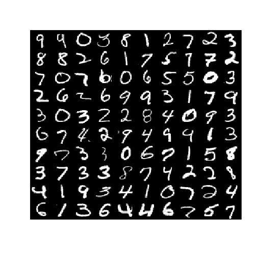28x28 visualization[

Dimension Reduction 1:

As we are having 784 features, which are prabably too many for training. We noticed the digits are well distinguishable, so that may be managable with lower resolution, say 28x28 to 14x14, which will significantly reduces the features from 784 to 196! The idea is to find the brightest pixel (max) within the adjance 2x2 grid.

  reduceDimfunction(data){
  posmatrix(1:784,28,28,byrow=T)
  offsetseq(1,28,2)
  n=0
  train.reduceddata.frame(index=1:nrow(data))
  if(!is.null(data$label)) train.reduced$labeldata$label
  data$labelNULL
  for (i in offset){
    for (j in offset){
      pxas.numeric(pos[i:(i+1),j:(j+1)])
      pxapply(data[,px],1,max)
      indexpaste0('px',n)
      n=n+1
      train.reduced[index]px
    }
  }
  train.reduced$indexNULL
  return (train.reduced)
}
train.reduced=reduceDim(train)
test.reduced=reduceDim(test)

Let’s take a look at the digit images after dimension reduction.

display(test.reduced[sample(28000,100),],14)

14x14 visualization

The digit is still well recognizable!

Dimension Reduction 2:

Besides the manual dimension reduction done earlier, we have a smarter alogrithm call ‘Principle Component Analysis’ (PCA). PCA is a method to compress the data and projected to n component axis. This comression and recovery process will incur some information loss, which is expressed the variance retained. In this case, we set the variance retrained to be 90%.

library(caret)
pcapreProcess(rbind(train.reduced,test.reduced),method='pca',thresh=0.9)
train.pcapredict(pca,train.reduced)
test.pcapredict(pca,test.reduced)

## 
## Call:
## preProcess.default(x = rbind(train.reduced, test.reduced), method =
##  "pca", thresh = 0.9)
## 
## Created from 70000 samples and 101 variables
## Pre-processing: principal component signal extraction, scaled, centered 
## 
## PCA needed 47 components to capture 90 percent of the variance.

With PCA implemented, we reduced the number of features to 47!

Train with Linear SVM:

For illustration purpose, we only trained 500 data points.

ctrltrainControl(method='cv',number = 10)
inTrain=sample(42000,500)
run_timesystem.time(fittrain(factor(label[inTrain])~.,data=train.pca[inTrain,],
            trControl = ctrl,
            method='svmLinear'))
print (fit)

## Support Vector Machines with Linear Kernel 
## 
## 500 samples
##  46 predictor
##  10 classes: '0', '1', '2', '3', '4', '5', '6', '7', '8', '9' 
## 
## No pre-processing
## Resampling: Cross-Validated (10 fold) 
## 
## Summary of sample sizes: 449, 452, 449, 449, 451, 450, ... 
## 
## Resampling results
## 
##   Accuracy   Kappa     Accuracy SD  Kappa SD  
##   0.8219855  0.801539  0.03704343   0.04130649
## 
## Tuning parameter 'C' was held constant at a value of 1
## 

Summary:

Simple linear SVM is giving fairely good accuracy with only small part of the entire training data. Further Explore Area:

1. Increase PCA threshold
2. Using higher order SVM / Gaussian Kernel SVM or Neural Network/Random Forest
3. Train with more data

The completed R code is available here.